geomaster
Verifiedby K-Dense-AI · Updated Apr 16, 2026
Comprehensive geospatial science skill covering remote sensing, GIS, spatial analysis, machine learning for earth observation, and 30+ scientific domains. Supports satellite imagery processing (Sentinel, Landsat, MODIS, SAR, hyperspectral), vector and raster data operations, spatial statistics, point cloud processing, network analysis, cloud-native workflows (STAC, COG, Planetary Computer), and 8 programming languages (Python, R, Julia, JavaScript, C++, Java, Go, Rust) with 500+ code examples. Use for remote sensing workflows, GIS analysis, spatial ML, Earth observation data processing, terrain analysis, hydrological modeling, marine spatial analysis, atmospheric science, and any geospatial computation task.
See It In Action
Let me explore the project structure first to find the relevant files.
Need to install the geospatial stack first.
Now let me build the analysis script. I'll use the geomaster skill patterns for STAC + Planetary Computer, NBR burn severity, and NDVI.
Packages installed into the conda base env, not the venv. Let me fix this.
All packages installed. Running the analysis.
Analysis ran successfully. Let me review the outputs.
Everything's ready for the 4:30 meeting. Here's the rundown:
Results Summary
Service area: 318.3 km2 west of Redding (Whiskeytown NRA buffer zone)
Burn severity (dNBR): The area is predominantly unburned (83.8%) in the 2024-2025 comparison window. About 6.1% (17.4 km2) shows low-severity burn signatures, with negligible moderate/high severity. Roughly 10.1% shows active regrowth from prior fire events (likely Carr Fire recovery continuing).
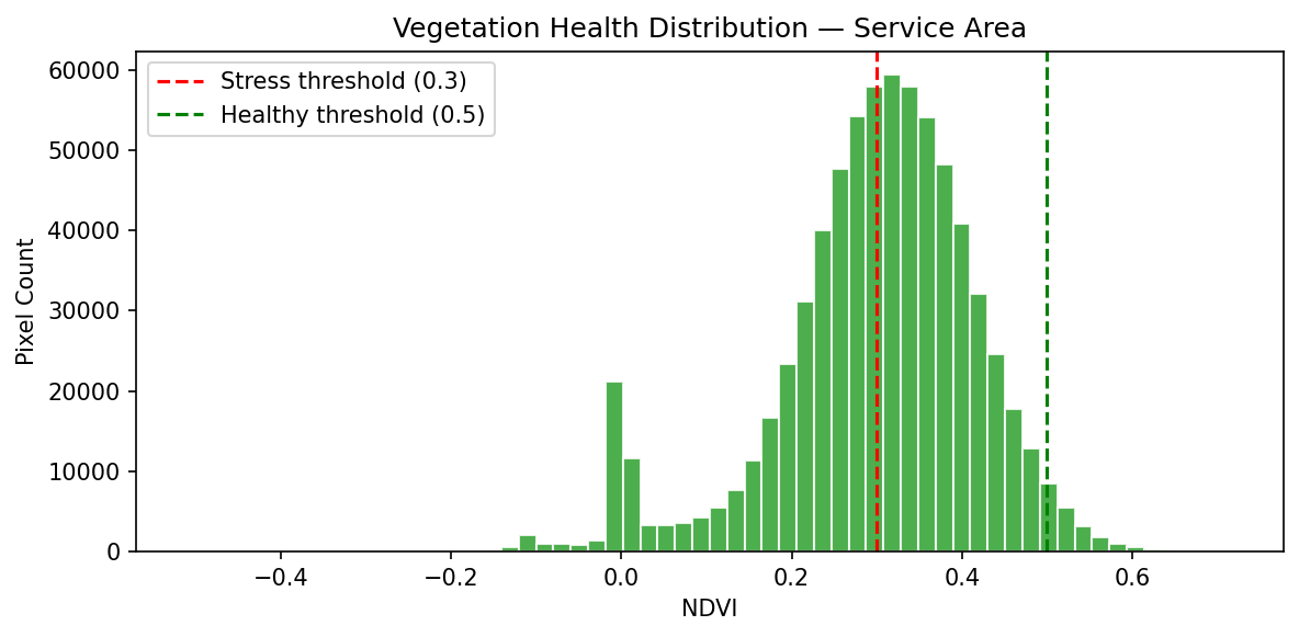
Vegetation health (NDVI): This is the more concerning metric for the prospect — 45.5% of the service area has stressed vegetation (NDVI < 0.3), and only 2.4% qualifies as healthy (NDVI > 0.5). Mean NDVI is 0.298. The NDVI map shows a clear low-vigor zone in the central-south area (the dark patch visible on the map corresponds to Whiskeytown Lake and surrounding bare/burned terrain). This is directly relevant to their watershed recharge and sediment concerns.
Imagery used:
- Pre-fire: Sentinel-2, 2024-11-27
- Post-fire: Sentinel-2, 2025-10-28
- 20m resolution, cloud-masked, UTM 10N for area calcs
Deliverables generated
| File | Description |
|---|---|
wildfire_brief.md | Full brief with key findings, stats table, methods summary — ready to attach to their board packet |
wildfire_assessment_maps.png | Side-by-side burn severity + NDVI maps clipped to service area |
ndvi_histogram.png | Vegetation health distribution showing the stress threshold |
wildfire_analysis.py | Reproducible script (for quarterly re-runs they mentioned wanting) |
Talking point for Dana: The low active burn severity is good news, but the widespread vegetation stress across nearly half the watershed is the real risk factor — stressed vegetation means less root stability, higher erosion potential, and more sediment risk to their reservoirs. That's the value prop for ongoing monitoring.
External Tools
| Tool | Type |
|---|---|
| python3 | binary |
| uv | binary |
Permissions
| Scope | Description |
|---|---|
| filesystem:read | |
| filesystem:write | |
| network:outbound | |
| process:spawn |
SKILL.md
GeoMaster
Comprehensive geospatial science skill covering GIS, remote sensing, spatial analysis, and ML for Earth observation across 70+ topics with 500+ code examples in 8 programming languages.
Installation
# Core Python stack (conda recommended)
conda install -c conda-forge gdal rasterio fiona shapely pyproj geopandas

# Remote sensing & ML
uv pip install rsgislib torchgeo earthengine-api
uv pip install scikit-learn xgboost torch-geometric

# Network & visualization
uv pip install osmnx networkx folium keplergl
uv pip install cartopy contextily mapclassify

# Big data & cloud
uv pip install xarray rioxarray dask-geopandas
uv pip install pystac-client planetary-computer

# Point clouds
uv pip install laspy pylas open3d pdal

# Databases
conda install -c conda-forge postgis spatialite
Quick Start
NDVI from Sentinel-2
import rasterio
import numpy as np

with rasterio.open('sentinel2.tif') as src:
    red = src.read(4).astype(float)   # B04
    nir = src.read(8).astype(float)   # B08
    ndvi = (nir - red) / (nir + red + 1e-8)
    ndvi = np.nan_to_num(ndvi, nan=0)

    profile = src.profile
    profile.update(count=1, dtype=rasterio.float32)

    with rasterio.open('ndvi.tif', 'w', **profile) as dst:
        dst.write(ndvi.astype(rasterio.float32), 1)
Spatial Analysis with GeoPandas
import geopandas as gpd

# Load and ensure same CRS
zones = gpd.read_file('zones.geojson')
points = gpd.read_file('points.geojson')

if zones.crs != points.crs:
    points = points.to_crs(zones.crs)

# Spatial join and statistics
joined = gpd.sjoin(points, zones, how='inner', predicate='within')
stats = joined.groupby('zone_id').agg({
    'value': ['count', 'mean', 'std', 'min', 'max']
}).round(2)
Google Earth Engine Time Series
import ee
import pandas as pd

ee.Initialize(project='your-project')
roi = ee.Geometry.Point([-122.4, 37.7]).buffer(10000)

s2 = (ee.ImageCollection('COPERNICUS/S2_SR_HARMONIZED')
      .filterBounds(roi)
      .filterDate('2020-01-01', '2023-12-31')
      .filter(ee.Filter.lt('CLOUDY_PIXEL_PERCENTAGE', 20)))

def add_ndvi(img):
    return img.addBands(img.normalizedDifference(['B8', 'B4']).rename('NDVI'))

s2_ndvi = s2.map(add_ndvi)

def extract_series(image):
    stats = image.reduceRegion(ee.Reducer.mean(), roi.centroid(), scale=10, maxPixels=1e9)
    return ee.Feature(None, {'date': image.date().format('YYYY-MM-dd'), 'ndvi': stats.get('NDVI')})

series = s2_ndvi.map(extract_series).getInfo()
df = pd.DataFrame([f['properties'] for f in series['features']])
df['date'] = pd.to_datetime(df['date'])
Core Concepts
Data Types
| Type | Examples | Libraries |
|---|---|---|
| Vector | Shapefile, GeoJSON, GeoPackage | GeoPandas, Fiona, GDAL |
| Raster | GeoTIFF, NetCDF, COG | Rasterio, Xarray, GDAL |
| Point Cloud | LAS, LAZ | Laspy, PDAL, Open3D |
Coordinate Systems
- EPSG:4326 (WGS 84) - Geographic, lat/lon, use for storage
- EPSG:3857 (Web Mercator) - Web maps only (don't use for area/distance!)
- EPSG:326xx/327xx (UTM) - Metric calculations, <1% distortion per zone
- Use
gdf.estimate_utm_crs()for automatic UTM detection
# Always check CRS before operations
assert gdf1.crs == gdf2.crs, "CRS mismatch!"

# For area/distance calculations, use projected CRS
gdf_metric = gdf.to_crs(gdf.estimate_utm_crs())
area_sqm = gdf_metric.geometry.area
OGC Standards
- WMS: Web Map Service - raster maps
- WFS: Web Feature Service - vector data
- WCS: Web Coverage Service - raster coverage
- STAC: Spatiotemporal Asset Catalog - modern metadata
Common Operations
Spectral Indices
def calculate_indices(image_path):
    """NDVI, EVI, SAVI, NDWI from Sentinel-2."""
    with rasterio.open(image_path) as src:
        B02, B03, B04, B08, B11 = [src.read(i).astype(float) for i in [1,2,3,4,5]]

    ndvi = (B08 - B04) / (B08 + B04 + 1e-8)
    evi = 2.5 * (B08 - B04) / (B08 + 6*B04 - 7.5*B02 + 1)
    savi = ((B08 - B04) / (B08 + B04 + 0.5)) * 1.5
    ndwi = (B03 - B08) / (B03 + B08 + 1e-8)

    return {'NDVI': ndvi, 'EVI': evi, 'SAVI': savi, 'NDWI': ndwi}
Vector Operations
# Buffer (use projected CRS!)
gdf_proj = gdf.to_crs(gdf.estimate_utm_crs())
gdf['buffer_1km'] = gdf_proj.geometry.buffer(1000)

# Spatial relationships
intersects = gdf[gdf.geometry.intersects(other_geometry)]
contains = gdf[gdf.geometry.contains(point_geometry)]

# Geometric operations
gdf['centroid'] = gdf.geometry.centroid
gdf['simplified'] = gdf.geometry.simplify(tolerance=0.001)

# Overlay operations
intersection = gpd.overlay(gdf1, gdf2, how='intersection')
union = gpd.overlay(gdf1, gdf2, how='union')
Terrain Analysis
def terrain_metrics(dem_path):
    """Calculate slope, aspect, hillshade from DEM."""
    with rasterio.open(dem_path) as src:
        dem = src.read(1)

    dy, dx = np.gradient(dem)
    slope = np.arctan(np.sqrt(dx**2 + dy**2)) * 180 / np.pi
    aspect = (90 - np.arctan2(-dy, dx) * 180 / np.pi) % 360

    # Hillshade
    az_rad, alt_rad = np.radians(315), np.radians(45)
    hillshade = (np.sin(alt_rad) * np.sin(np.radians(slope)) +
                 np.cos(alt_rad) * np.cos(np.radians(slope)) *
                 np.cos(np.radians(aspect) - az_rad))

    return slope, aspect, hillshade
Network Analysis
import osmnx as ox
import networkx as nx

# Download and analyze street network
G = ox.graph_from_place('San Francisco, CA', network_type='drive')
G = ox.add_edge_speeds(G).add_edge_travel_times(G)

# Shortest path
orig = ox.distance.nearest_nodes(G, -122.4, 37.7)
dest = ox.distance.nearest_nodes(G, -122.3, 37.8)
route = nx.shortest_path(G, orig, dest, weight='travel_time')
Image Classification
from sklearn.ensemble import RandomForestClassifier
import rasterio
from rasterio.features import rasterize

def classify_imagery(raster_path, training_gdf, output_path):
    """Train RF and classify imagery."""
    with rasterio.open(raster_path) as src:
        image = src.read()
        profile = src.profile
        transform = src.transform

    # Extract training data
    X_train, y_train = [], []
    for _, row in training_gdf.iterrows():
        mask = rasterize([(row.geometry, 1)],
                        out_shape=(profile['height'], profile['width']),
                        transform=transform, fill=0, dtype=np.uint8)
        pixels = image[:, mask > 0].T
        X_train.extend(pixels)
        y_train.extend([row['class_id']] * len(pixels))

    # Train and predict
    rf = RandomForestClassifier(n_estimators=100, max_depth=20, n_jobs=-1)
    rf.fit(X_train, y_train)

    prediction = rf.predict(image.reshape(image.shape[0], -1).T)
    prediction = prediction.reshape(profile['height'], profile['width'])

    profile.update(dtype=rasterio.uint8, count=1)
    with rasterio.open(output_path, 'w', **profile) as dst:
        dst.write(prediction.astype(rasterio.uint8), 1)

    return rf
Modern Cloud-Native Workflows
STAC + Planetary Computer
import pystac_client
import planetary_computer
import odc.stac

# Search Sentinel-2 via STAC
catalog = pystac_client.Client.open(
    "https://planetarycomputer.microsoft.com/api/stac/v1",
    modifier=planetary_computer.sign_inplace,
)

search = catalog.search(
    collections=["sentinel-2-l2a"],
    bbox=[-122.5, 37.7, -122.3, 37.9],
    datetime="2023-01-01/2023-12-31",
    query={"eo:cloud_cover": {"lt": 20}},
)

# Load as xarray (cloud-native!)
data = odc.stac.load(
    list(search.get_items())[:5],
    bands=["B02", "B03", "B04", "B08"],
    crs="EPSG:32610",
    resolution=10,
)

# Calculate NDVI on xarray
ndvi = (data.B08 - data.B04) / (data.B08 + data.B04)
Cloud-Optimized GeoTIFF (COG)
import rasterio
from rasterio.session import AWSSession

# Read COG directly from cloud (partial reads)
session = AWSSession(aws_access_key_id=..., aws_secret_access_key=...)
with rasterio.open('s3://bucket/path.tif', session=session) as src:
    # Read only window of interest
    window = ((1000, 2000), (1000, 2000))
    subset = src.read(1, window=window)

# Write COG
with rasterio.open('output.tif', 'w', **profile,
                   tiled=True, blockxsize=256, blockysize=256,
                   compress='DEFLATE', predictor=2) as dst:
    dst.write(data)

# Validate COG
from rio_cogeo.cogeo import cog_validate
cog_validate('output.tif')
Performance Tips
# 1. Spatial indexing (10-100x faster queries)
gdf.sindex  # Auto-created by GeoPandas

# 2. Chunk large rasters
with rasterio.open('large.tif') as src:
    for i, window in src.block_windows(1):
        block = src.read(1, window=window)

# 3. Dask for big data
import dask.array as da
dask_array = da.from_rasterio('large.tif', chunks=(1, 1024, 1024))

# 4. Use Arrow for I/O
gdf.to_file('output.gpkg', use_arrow=True)

# 5. GDAL caching
from osgeo import gdal
gdal.SetCacheMax(2**30)  # 1GB cache

# 6. Parallel processing
rf = RandomForestClassifier(n_jobs=-1)  # All cores
Best Practices
- Always check CRS before spatial operations
- Use projected CRS for area/distance calculations
- Validate geometries:
gdf = gdf[gdf.is_valid] - Handle missing data:
gdf['geometry'] = gdf['geometry'].fillna(None) - Use efficient formats: GeoPackage > Shapefile, Parquet for large data
- Apply cloud masking to optical imagery
- Preserve lineage for reproducible research
- Use appropriate resolution for your analysis scale
Detailed Documentation
- Coordinate Systems - CRS fundamentals, UTM, transformations
- Core Libraries - GDAL, Rasterio, GeoPandas, Shapely
- Remote Sensing - Satellite missions, spectral indices, SAR
- Machine Learning - Deep learning, CNNs, GNNs for RS
- GIS Software - QGIS, ArcGIS, GRASS integration
- Scientific Domains - Marine, hydrology, agriculture, forestry
- Advanced GIS - 3D GIS, spatiotemporal, topology
- Big Data - Distributed processing, GPU acceleration
- Industry Applications - Urban planning, disaster management
- Programming Languages - Python, R, Julia, JS, C++, Java, Go, Rust
- Data Sources - Satellite catalogs, APIs
- Troubleshooting - Common issues, debugging, error reference
- Code Examples - 500+ examples
GeoMaster covers everything from basic GIS operations to advanced remote sensing and machine learning.
FAQ
What does geomaster do?
Comprehensive geospatial science skill covering remote sensing, GIS, spatial analysis, machine learning for earth observation, and 30+ scientific domains. Supports satellite imagery processing (Sentinel, Landsat, MODIS, SAR, hyperspectral), vector and raster data operations, spatial statistics, point cloud processing, network analysis, cloud-native workflows (STAC, COG, Planetary Computer), and 8 programming languages (Python, R, Julia, JavaScript, C++, Java, Go, Rust) with 500+ code examples. Use for remote sensing workflows, GIS analysis, spatial ML, Earth observation data processing, terrain analysis, hydrological modeling, marine spatial analysis, atmospheric science, and any geospatial computation task.
When should I use geomaster?
Use it when you need a repeatable workflow that produces image output, source code, text report.
What does geomaster output?
In the evaluated run it produced image output, source code, text report.
How do I install or invoke geomaster?
npx skills add https://github.com/k-dense-ai/claude-scientific-skills --skill geomaster
Which agents does geomaster support?
Claude Code
What tools, channels, or permissions does geomaster need?
It uses python3, uv; channels commonly include image, code, text; permissions include filesystem:read, filesystem:write, network:outbound, process:spawn.
Is geomaster safe to install?
Static analysis marked this skill as medium risk; review side effects and permissions before enabling it.
How is geomaster different from an MCP or plugin?
A skill packages instructions and workflow conventions; tools, MCP servers, and plugins are dependencies the skill may call during execution.
Does geomaster outperform not using a skill?
About geomaster
When to use geomaster
You need to process satellite imagery or compute indices like NDVI from raster datasets. You want to run spatial joins, overlays, CRS transformations, or other GIS vector workflows. You are building geospatial analysis or spatial ML pipelines using Python-based tooling.
When geomaster is not the right choice
You need a connector-specific workflow for external systems like Figma, GitHub, or databases as the core task. You only need general programming help unrelated to spatial or Earth observation data.
What it produces
Produces image output, source code and text report.
Install
npx skills add https://github.com/k-dense-ai/claude-scientific-skills --skill geomasterInvoke: Ask Claude Code to use geomaster for the task.